Sparse Index Pattern
May 9, 2026Introduction
A query that should take seconds is taking 15 minutes. Your batch job that used to take a few hours is now taking 24–48 hours. You add more nodes to the cluster. It gets worse. You try to parallelize the requests in the batch job and end up hammering the OLAP cluster. Almost all of your queries start timing out. This is not a hardware problem. This is a data structure problem.
The query causing the failure looks something like this:
SELECT COUNT(DISTINCT user_id) FROM T
WHERE advertiser_id = {...}
AND event_date IN ({past m days})
AND event_name IN ({dynamic list of events})
T is large — well over 100 million rows — and the list of event names is
dynamic and arbitrary, ruling out pre-computing answers for every possible input. The input space is
exponentially large.
In this article, we introduce the Sparse Index Pattern: a pre-aggregation technique that exploits the sparsity of real-life data to reduce query cost from O(N) in raw event volume to O(S) in distinct behavioral sequences — where N may be hundreds of millions and S is typically no more than a few dozen. In practice, this takes queries that run for minutes under load and brings them to milliseconds, independent of scale. This pattern was developed to address a production failure impacting ad systems at scale — the problem and solution described here are real, not theoretical.
Naive Solution
We can always submit a request with this query to your typical OLAP: Amazon Athena, Redshift, Presto, Snowflake, etc. But it is slow, doing a scan, and the query may get queued. So you end up waiting up to a couple minutes for a result. What’s worse, if running this query with high QPS (for example, as part of a batch job), the OLAP cluster fails under stress, that couple-minute latency may turn into 10–15+ minute latency, and you begin to get cascading failures. Imagine you may be doing parallel queries as well. For instance, you want the answer for the past 1/7/30/60/180 days, so you fire these queries in parallel. In addition, your data (number of advertisers) begins to scale, so waiting minutes for every request prevents your batch processing from finishing on time.
If this is an important part of your system, the entire system begins to fail.
The “Scaling Trap”: Why More Hardware Fails
There are a few things we might try. Unfortunately they all lead to a dead end.
- Scale the OLAP cluster horizontally: add more nodes to your OLAP cluster, but this only solves for aggregate throughput, not per-query physics. You are still stuck paying for a linear scan. As your traffic increases, you may find yourself paying a 10x cost for a 20% improvement in stability.
- Cache all the data in memory and do the aggregations in memory: this avoids the queueing issue. This is a mistake. OLAP engines are some of the most heavily optimized software in existence (vectorized execution, columnar compression, hardware-level parallelism). Thinking you’ll beat them with application-layer for-loops is a category error. You cannot out-process the database’s own engine at its own game.
- If it’s a batch job, shard the job: create n concurrent job instances, each processing (1/n)th of the traffic. This is the most dangerous of the three solutions. You aren’t just splitting the work, you are multiplying the contention. Instead of one heavy query, you are now hammering the cluster with n concurrent requests. This leads to resource starvation: the workers spend more time context-switching and fighting for memory slots than actually scanning data. The result is an “OLAP Death Spiral” — queueing times skyrocket, and the entire system eventually collapses under cascading failures.
Implementation Context
In this article, we assume an AWS technology stack, but the problem itself is transferable to whatever your stack is; all the AWS-specific details are not critical to understand the pattern.
Suppose we store advertiser event data in a database — either SQL or NoSQL; we’ll assume DynamoDB in our context. Further assume that we have daily or hourly offline copies available for analysis in a data warehouse. This could be implemented with batch jobs from the main table or in streaming fashion. We’ll use Spark for pre-aggregation, S3 for intermediate storage, and DynamoDB for the fast index layer.
Sparse Index Pattern: The Optimal Solution
Instead of trying to get clever with scaling the OLAP interface, we should recognize OLAP tools
are not designed for online (OLTP) querying. So what we do is pre-aggregate our data in a queryable
way. Again, we can’t pre-compute the answer for every query. But we can group by
advertiser_id and user_id to compute the list of events on that
user’s journey (also group by query_window, which represents the last n
days). This is partly useful. But we still end up with a huge table (remember, T has
>> 100m rows). Instead of grouping by the user_id, we group by the list of events
(in this case, we don’t care about duplicate events or order, so we can canonicalize by sorting
the events; in other cases, order or duplicates may matter) and store the frequency at which we see
that sequence. Remember, we don’t care about actual user ids here, only how many distinct users
hit a certain event sequence.
Now, we can fetch all the rows for a specific advertiser and simply compute set intersections (of the event lists we retrieve and the dynamic input event list), and sum up the frequencies of sets that intersect.
This is a big improvement, but we are still querying our OLAP system, and still have the problem of queued queries, slow results, and so on.
So we copy the results of this pre-aggregation pipeline into a fast index. Assume the pre-aggregation output is stored in S3. We can copy this into a DynamoDB table as our index (again, other DB systems will work for this as well). DynamoDB with the appropriate schema will let us do range queries to quickly fetch all the data.
In the name here, we are using the word sparse. This is because we are indexing not user journeys, but rather behavioral entropy. This is very sparse. You can think of the 80/20 principle, but much more extreme. In an advertiser funnel, where the top-funnel event is something like “PageView,” you may find that you have millions of users who just hit “PageView” but nothing downfunnel from that. In practice, even if you have 50 different possible events for one advertiser, you may end up with only dozens (or possibly hundreds) of distinct event sets (even if you have millions of events for that advertiser). Nowhere near the theoretical maximum of .
This means if we have the right index schema set up, we can fetch the data in one range query and do the set intersections and frequency summing in memory. (We can even do it with a filter expression in DynamoDB and save our application-level hosts’ memory, but then you lose control over tuning the CPU/memory profile where you do the calculations. That is a fine detail that can be determined based on your use case.)
DynamoDB Details
First, how do we get the data from our S3 pipeline output into DynamoDB? We can just have a simple batch job (for example, AWS Batch). Even a Lambda would likely be fine (though a bit riskier due to memory/runtime limitations). Recall that the pre-aggregated table will be much smaller. The exact numbers depend on your data, but per query window, you’ll likely see << 1 million rows even when your event table has hundreds of millions of rows of data. For this job, either use PayPerRequest billing mode, or pre-provision your table for high WCU (before the job, then dial it down after).
Index rebuilds should follow a blue-green deployment pattern. Rather than writing directly to the live table, write the new index to a separate inactive table. Once the build is complete and validated, atomically swap the pointer your application uses to reference the active table. This ensures that readers always see a fully consistent index — either the previous version or the new one, never a partial write. The old table can be deleted or retained for rollback purposes depending on your operational requirements.
Including the pre-aggregation pipeline (whether using Spark or other tools), you should be able to build the DynamoDB index (note: this is a regular DynamoDB table, which we are viewing as an index; we are not referring to DynamoDB LSIs or GSIs) end-to-end in under half an hour.
Now let’s discuss the schema itself. This will be a single-table design, and can be translated to other NoSQL DB systems if you use a different stack for your indexing. There are a few different shapes for your partition key, and we will make use of sort keys for efficient range queries. The partition key will be a string and the sort key will be a number.
Specifically, the sort key will be a row number, which lets us fetch either all rows, or do pagination as desired (or if the data volume requires it). Partition keys:
EventMapping:advertiser_id:query_windowEventListWithFrequency:advertiser_id:query_windowEventListCount:advertiser_id:query_window
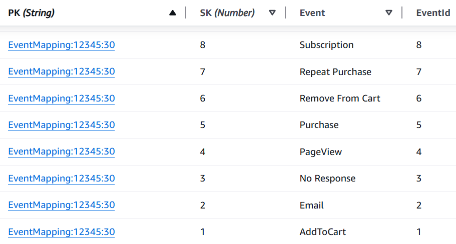
The first partition key type, EventMapping:advertiser_id:query_window, will store a
mapping such as PageView → 1. This can be done with an “Event”
attribute (a string) and an EventId attribute (an integer).
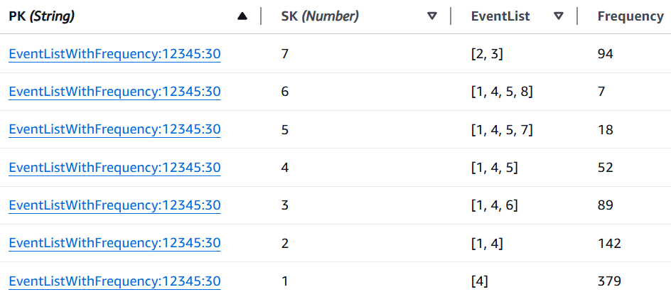
The second partition key type, EventListWithFrequency:advertiser_id:query_window,
will store an “EventList” attribute (either a string to be deserialized application-side
or a list/set of integers) and a “Frequency” attribute (an integer).
The third partition key type, EventListCount:advertiser_id:query_window, will store
a “RowCount” attribute (an integer). This tells us how many distinct event sequences
there are in our index (per advertiser/query window). In rare cases where we might need or want to
paginate, this lets us avoid synchronous pagination and fetch multiple pages of data in parallel (if
desired). We could similarly store the number of event mappings with another partition key type, but
this is very likely unnecessary. The number of distinct events for an advertiser will almost never
be more than a few hundred. We could also keep the EventMappings as one item/row and
simply store the map (of all events) in an attribute and avoid the need for a range query, but for
this write-up, we will stick with one mapping per row (which may be better for rare cases with
advertisers with many events with long names, breaking the 400 KB item-size limit).
For simplicity, we’ll ignore the EventListCount:advertiser_id:query_window
partition key and ignore pagination details, but those are easy to add into a system. If you
determine you want to pull no more than 10,000 rows at once, for example, simply get the number of
rows, break the row count into a set of disjoint ranges of length at most 10,000, and issue the
page fetches (possibly in parallel). For example, if there are 23,000 rows, your disjoint ranges
will be (1, 10000), (10001, 20000), and (20001, 23000). However, in practice, you won’t see
more than a few hundred rows of data due to the sparsity of real-life data outside of very rare
cases.
What the Index Looks Like
Below is what these two partition key types look like in DynamoDB for advertiser 12345 over a 30-day window.
Event mappings — each event name assigned a stable integer ID:
Event lists with frequencies — each distinct behavioral sequence and the number of users who followed it:
Index Query Latency and Size
Assuming you query from DynamoDB in the same region/AZ as the table, everything will be very low-latency. In general, the full API (all data fetches needed, plus the in-memory intersection calculations) will complete in under 20 ms. In addition, because DynamoDB (or whichever NoSQL DB you choose as your index) is designed for high throughput, it will scale to however much concurrent traffic you need. You no longer have a single point of failure that easily gets overwhelmed in your system (the OLAP cluster).
Because the index will be so small (see below), it will likely hit DynamoDB’s SSD storage. It could even be loaded up in your application hosts’ cache, or you could stick DAX or Redis on top of your indexing setup for lower latency. If you store it locally in your application, you will be able to serve requests in under 1 ms. But if you get into streaming updates instead of periodic batch jobs (whether daily or hourly), cache invalidation becomes more complicated.
In addition, your index will be very small and achieve sub-linear growth. Even if your upstream event data has hundreds of millions of rows, you likely have << 1M rows per query window. Your index is unlikely to even exceed 1 GB. This of course depends on your actual data, whether you group on anything else (like ad id, etc.).
As an illustrating example, suppose one day one million different users, all from a bot farm, view an ad for an advertiser, triggering the “PageView” event, but trigger nothing downfunnel. The event list [“PageView”] almost certainly already existed in the data. Even though you get 1 million new rows in your events table, this adds zero new rows to the index. It simply increases the Frequency attribute by 1 million. This architectural decoupling ensures that the cost of retrieval is a function of behavioral entropy, not raw event cardinality.
One fine point: why did we add EventMappings? It losslessly compresses the data we
want to store, which means storage requirements and network transfer requirements are much lower.
It is cheaper to store integer lists like [1, 2, 3] than string lists like
["PageView", "AddToCart", "Purchase"], especially if the strings are even longer. In
fact, one can optimize even further and use an integer instead of a list and simply treat the
integer as a bitmask/bitmap. This is part of what helps keep the index size so small.
Geometric Visualization
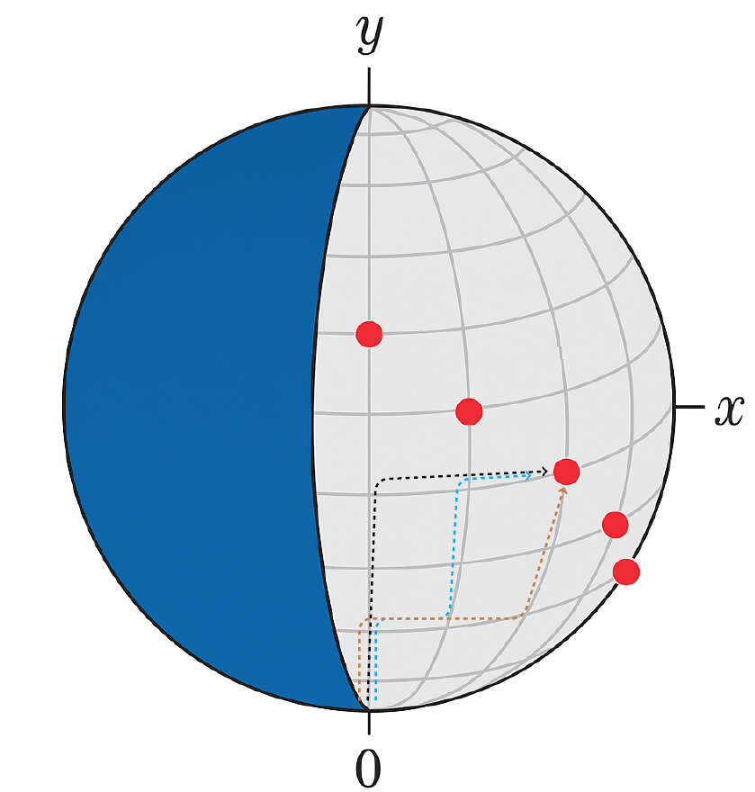
We can visualize this with geometry by modeling event sets as elements of the binary space . This space forms a -dimensional hypercube, and any event set corresponds to a path from the origin to another point — by flipping up to bits. To visualize this, we can project onto a lattice on the boundary of a sphere.
Starting at the origin, for each bit:
- 0 → move right
- 1 → move up
Every binary string defines a unique right/up lattice path of length , and ends at a point such that . There are precisely such paths — one for each event sequence. The number of paths ending at is . Note that .
In the image above, each red point corresponds to a set of cardinality-y event sequences. Each path corresponds to an event sequence. We draw a few to illustrate this. In our example, (meaning there are 6 different events).
The red point with paths coming towards it represents the set of event sequences with 4 different events:
- Black path: [Event1, Event2, Event3, Event4]
- Blue path: [Event1, Event2, Event4, Event5]
- Brown path: [Event1, Event2, Event5, Event6]
Only a narrow set of paths to points on a diagonal line (the line ) forming a triangular subsection of the full lattice are realized event sequences. The rest of the space is empty. This illustrates how sparse our data is.
Extensions
Below I discuss a few extensions of this design pattern.
Optimizing Latency
In the pattern above, we simply made range queries to DynamoDB (or a similar system). This is good enough to achieve under 20 ms latency. If we want additional speed, we can set up DAX or Redis/ElastiCache on top of the DB/index layer. In fact, we could just load the data into memory on the hosts periodically since the full index is likely to be quite small, considering the sparsity of real-life data. For example, even with hundreds of millions of rows, we may have << 1 million rows in our table. This would translate to ~1 ms latency. This does get a bit more complex if strongly consistent data is required (see streaming indexing below).
Event List Format
Above, we assumed a list/set of integers to store the data we need. This can be made more efficient with a bitmask (assuming there are no more than 64 distinct events). But even with more events, we can use bitmaps.
Streaming Indexing
If we want to have our index reflect changes more immediately than a batch job would provide, the challenge is that the batch index stores aggregate counts, not individual user records. When a new event arrives for a user, we need to know which sequence they were previously in to correctly decrement that count and increment the new one — but that information isn’t in the index. This requires maintaining a small amount of per-user state in the streaming layer, separate from the aggregate index.
Assume that our main table that houses events is a DynamoDB table, and that we re-build our index hourly. Set up a DynamoDB stream on this table (if not DynamoDB, use Kinesis/Kafka) that triggers a Lambda. For each event, we need the current sequence for that advertiser and user. We don’t want to store millions of user sequences in DynamoDB. So instead, use a bloom filter to check if we’ve seen this user in the last hour. If so, pull their “stream-only” sequence from a small DynamoDB table (or Redis).
When we want to query for an advertiser, check the batch count (e.g., the sequence [1, 2] has
1000 distinct users). Then query the streaming delta. To avoid double-counting, the streaming state
must track “transition” users. If user A moves from [1, 2] to [1, 2, 3], the streaming
logic must return [1, 2]: -1 and [1, 2, 3]: +1.
We treat the batch index as immutable and the streaming layer as an override. At query time:
- Fetch count for [Sequence X] from the batch index DynamoDB table.
- Fetch
delta_countfor [Sequence X] from the streaming DynamoDB. - The result is then the sum of the count and
delta_count.
How is the delta maintained? When a streaming event arrives for user A:
- Look up user A’s sequence in the S3 data for the batch index row (by storing the list of users for that sequence in the underlying S3 storage).
- If user A was in [Event1, Event2], and the new event is Event3, then decrement the delta for [1, 2] and increment the delta for [1, 2, 3].
Is this scalable? This streaming approach is definitely heavier, and for most use cases, you won’t need real-time sequence updates, and even a simpler streaming solution that doesn’t handle double-counting gives a reasonable approximation. But if we do need exactness, we should still be able to handle updates that are not stale by more than, say, 30–60 seconds.
One fine point specific to the streaming layer: if a streaming event arrives with an event name that has never been seen before, it must be assigned a new integer ID before the sequence can be updated. In a distributed streaming environment this assignment needs to be atomic — two concurrent stream processors receiving the same novel event must not assign it different IDs. A conditional write to DynamoDB handles this. The consequence worth noting is that new IDs are assigned in order of first appearance, so the canonical sort order of event sets — which is by ID — will not be alphabetical by event name. This is not a correctness issue, since the sort order only needs to be consistent, not human-readable. But it is an operational detail: if you ever need to inspect the index directly, you will need the event mapping table to interpret it.
Other Aggregations
In this article, we assumed we are looking for counts/frequencies. We can also ask about:
- The sum of some value (e.g., total revenue from users who followed this sequence)
- Set of user IDs (answer exact membership questions)
- Max/min of some metric (e.g., what’s the highest LTV user following this event path?)
- Arbitrary aggregate: anything that can be computed incrementally and merged over disjoint sets
The sequence index naturally forms a trie structure over the event space. This opens up more complex query patterns — for instance, range queries over metric values along behavioral paths. This also connects to the classical equivalence between RMQ (range minimum query) and LCA (lowest common ancestor). Whether the added complexity is necessary depends on your use case, but the structure supports it.
Other Contexts
Throughout this article, we framed everything through the lens of ads. But this is a general concept that can be applied in many domains.
RAG / LLM Orchestration Efficiency. You might be interested in RAG / LLM
orchestration efficiency. Did your LLM answer a question correctly by calling two tools, or by
calling a convoluted sequence of 15 tools? You might ask how many chat sessions required exactly two
clarifications before a successful response, or how many agentic runs that called the search tool
more than 3x still failed to produce a satisfactory answer. Even across billions of LLM
interactions, the number of distinct orchestration patterns will be relatively small. In this case,
query by model_id or agent_type instead of advertiser_id.
Google Search / Autosuggest. Think of raw events as search queries (normalized, through something like BM25 / NLP). The behavioral sequences are the paths users take through a search session. Perhaps someone went along this search pattern: [NBA scores] → [Los Angeles Lakers score] → [LeBron James stats]. Autosuggest should anticipate the next step.
The sparse index answers “how many users who searched X subsequently searched Y” efficiently at scale, which can be useful for sequence-aware autosuggest. Despite billions of searches, the number of distinct meaningful two- or three-step search sequences will be relatively small. In this case, query by search sequence prefix (using 1–2 search terms).